Neural Nets from Scratch

2026-01-19

This post is part of a series that intends to distil what I've learned while interviewing at the world's top AI labs. Though the ML field has been well established for several decades, the business of AI today writ large is next token prediction. At the very heart of this process lies the Neural Network and it's variants that undergird the likes of ChatGPT, Gemini and Claude. This post aims to communicate the fundamentals of training a network on tabular data and image data. Subsequent posts will focus on sequential data prediction using the recurrent nets and the fabled Transformer. I assume familiarity with common ML nomenclature, including concepts like layers, neurons and other basic terminology.

Multilayer Perceptrons

To start with, let us motivate the problem from the ground up. Suppose we have some dataset $\mathbf{X} \in \mathbb{R}^{N \times F}$ where $N$ represents the number of of examples and $F$ represent the size of the feature vector. We also have some corresponding labels for this data $\mathbf{Y} \in \mathbb{Z}^{N \times K}$ where $K$ is the number of possible output variables. Our goal is to predict, given some new data $X_{new}$, an appropriate label $P(\hat{Y}|X_{new})$. As a concrete example, suppose $F=2, K=2$ and $Y$ is a one-hot encoded variable corresponding to 1-of-K class labels. This is a classic problem in ML literature that can be solved in a number of ways. Figure \ref{fig:wayve_classification} illustrates this example with two different datasets. The one on the left shows a straightforward supervised classification problem where a decision boundary can be determined directly in the original feature space. The second plot illustrates a slightly more complex problem that requires some transformation in the feature space to determine the a linear decision boundary. I leave it to the reader to determine what is an appropriate choice.

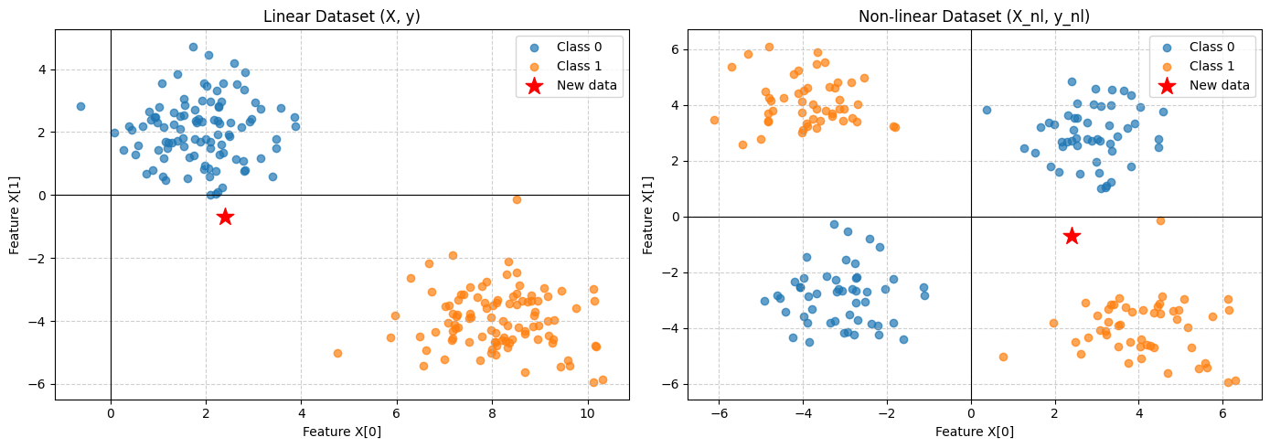
Simple 2D linear classification — Figure 1. Typical classification problem with 2 different datasets.

After some thought, it should be clear what an appropriate feature transformation is. The question remains, however, of what to do when the datasets are more complex with highly nonlinear features. How should we determine the transformation? Similarly, we have constrained the problem to two dimensions for ease of visualisation. In anything more than three dimensions, our intuition breaks down and determining the feature representation becomes exponentially more difficult. These represent the primary motivations of the Multilayer Perceptron (MLP). MLPs or Feedforward Neural Networks address this problem by learning a feature vector $\phi(X)$ from the data by fixing the total number of parameters but allowing them to be adaptive during training.

Forward pass

Given the data $(\mathbf{X}, \mathbf{Y})$, the goal of a MLP is to learn a model that maximises $p_{\theta}(\mathbf{Y}|\mathbf{X})$. The first step to achieving this is to compute its prediction of $\hat{Y}$ given the data, known as the forward pass. Suppose our network has two hidden layers followed by an output layer. Each hidden layer represents a nonlinear affine transformation of its input, represented as:

$$ \mathbf{a} = \mathbf{X} \cdot \mathbf{\Theta} + \theta_b $$

$$ \mathbf{z} = f(\mathbf{a}) $$

The dot product between $\mathbf{X}$ and $\mathbf{\Theta} \in \mathbb{R}^{F \times H_1}$ produces $H_1$ neurons in the first hidden layer, $\mathbf{a} \in \mathbb{R}^{N \times H_1}$ for $N$ examples. A bias term is also usually added to each neuron, $\theta_b \in \mathbb{R}^{H_1}$. The final output of the first hidden layer, $\mathbf{z}$, is produced via an elementwise nonlinear activation function $f()$. The choice of activation is problem dependent though ReLU is a common choice in most state of the art models. For the next hidden layer with $H_2$ neurons, this process is repeated again. The final output layer also consists of an affine transformation with a task dependent activation function $g()$, shown below. For a regression task, $g()$ is just the identity function. For a binary or multiclass classification problem, $g()$ is sigmoid or softmax function respectively.

$$ \mathbf{a}_{out} = \mathbf{z} \mathbf{\Theta}_{out} + \theta_{out,b} $$

$$ \mathbf{\hat{y}} = g(\mathbf{a}_{out}) $$

In our example of a network with 2 hidden layers, 2D features with 2 output classes, the forward pass would look something like:

import numpy as np
from typing import List 
def forward(x, weights: List[np.ndarray], biases:List[np.ndarray], task= "BCE"):

    for i, (w, b) in enumerate(zip(weights, biases)):
        a = np.einsum("bf,fh->bh", x, w) + b
        if  i < len(weights)-1:
            #hidden layer ReLU activation
            x = np.where(a>0, a,0)
        else:
            x = a

    if task == "regression":
        # no activation 
        y_hat = x 
    elif task == "BCE":
        #sigmoid 
        y_hat = 1 / (1+ np.exp(-1*x))
    else:
        raise NotImplementedError("Only regression and BCE loss is supported for now")
    
    return y_hat

The code block above shows two distinct stages. The first executes the affine transformations using np.einsum (Tim Rocktaschel has a great blog post about it). The second stage takes the vector $\mathbf{a_out} \in \mathbb{R}^{N \times K}$ and applies a task specific activation, producing our predictions $\hat{Y}$.

Loss Functions

To train our network, we need to determine some measure of performance. Earlier, we mentioned that the goal is to learn a model $p_{\theta}(\mathbf{Y}|\mathbf{X})$. What would be a good method to select a set of parameters $\mathbf{\Theta}$ from the space of all possible values that would constitute a good model? The most widely used technique to achieve this is called Maxmim Likelihood Estimation (MLE). Going down the rabbit hole that is MLE, you will start to uncover fascinating relationships with concepts like information content (entropy) and KL-divergence. For the purpose of this post, however, it is sufficient to know that MLE describes a principled way to derive task specific loss functions. Perhaps a future blog post will provide a detailed derivation that begins with $\text{argmax}_{\theta} p_{\theta}(\mathbf{Y}|\mathbf{X})$ and ends up with:

$$ E(\theta) = \frac{1}{N} \sum_{i=1}^N \Big( \hat{Y}_i - t_i \Big )^2 \text{ or } E(\theta) = -\frac{1}{N} \sum_{i=1}^N t_i \text{ln}\hat{y}_i + (1-t_i)\text{ln}(1- \hat{y}_i) $$

representing the 1D regression and Binary Cross Entropy (BCE) loss. The variables $\hat{y}_i$ and $t_i$ refer to our network prediction and target variable respectively. We can compute our loss for a batch of size $N$ as:

def compute_loss(pred, target, task="BCE"):

    N, K = pred.shape
    if task == "BCE":
        eps = 1e-7
        pred = np.clip(pred, eps, 1 - eps)  # Prevent log(0)
        loss = - np.sum((target*np.log(pred) + (1-target)*np.log(1-pred))) * 1/N
        
    elif task =="regression":
        loss = np.sum((pred - target)**2) * 1/N # for k=1
    else:
        raise NotImplementedError("Only regression and BCE loss is supported ")

    return loss

Error Backpropagation

The secret sauce of training a NN is based on the technique of Backprop, where the deriviatives of the error with respect to all the weights, $\Theta$, is determined using the Chain Rule in multivariate calculus. The goal is determine the gradient of the error with respect to each weight and bias term, $\frac{\partial E}{\partial W_i} \text{ and } \frac{\partial E}{\partial b_i} $. For the weights in the last layer, the gradient can be computed as:

$$ \frac{\partial E}{\partial W_{ko}} = \frac{\partial E}{\partial \hat{y}_k} \cdot \frac{\partial \hat{y}_k}{\partial a_k} \cdot \frac{\partial a_k}{\partial W_{ko}} $$

Recall that the output is determined by the following equations:

$$ \hat{y}_k = g(a_k) $$ $$ a_k = \mathbf{z}^{(2)} \cdot \mathbf{W}_{ko} + b_{ko} $$

where $\mathbf{z}^{(2)}$ denotes the activation vector from the previous layer. The error term $E$ corresponds to the task specific loss functions described above. For a regression task $g()$ is just the identity, with the derivative $\frac{\partial \hat{y}_k}{\partial a_k} = 1$. For the binary classification task, $\frac{\partial \hat{y}_k}{\partial a_k}$ is the derivative of the sigmoid function wrt $a_k$.

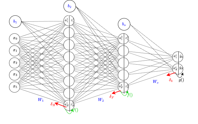
Let's introduce a variable $\delta_j = \frac{\partial E}{\partial a_j} $ for the j-th layer in the network. The key idea in backpropogation is to determine the value of this vector at each layer, with its size being equal to the number of neurons in layer $j$. This is depicted in the diagram below as $\delta_H, \delta_F, \text{ and } \delta_k$. If we can calculate what each of these vectors are, then computing the gradient wrt to the weight matrix $W_j$ becomes relatively straightforward.

Visualisation of errors backpropagating through the network — Figure 2. Backpropagation of errors through a network.

The classification and regression settings are almost idenitical, with the main difference occurring in the final layer due to the activation function $g()$. For simplicity, we will begin with the regression setting first and backprogate through the network, layer by layer.

Output Layer

$$ \delta_k = \frac{\partial E}{\partial \hat{y}_k} \cdot \frac{\partial \hat{y}_k}{\partial a_k} = \frac{1}{N} \Big( \hat{Y}_{ik} - t_{ik} \Big ) $$

The more precocious reader will note that for any task, regression or (binary/mulitple) classification, the term $\delta_k$ is identical. This is because the product of $ \frac{\partial E}{\partial \hat{y}_k} \cdot \frac{\partial \hat{y}_k}{\partial a_k}$ in any classification setting also reduces to the expression shown above. A BCE output is trivial to compute when you know the derivative of the sigmoid. Eli Bendersky has an excellent blog post on the more complex cross-entropy setting that requires the Jacobian of the softmax function.

This bias term is the easiest to start with since $\frac{\partial a_k}{\partial b_{o}} =1$. We just sum across the batch dimension: $$ \frac{\partial E}{\partial b_{o}} = \sum^N \delta_k $$

We know the shape of is $W_o \in \mathbb{R}^{F \times K}$, so we need to ensure that our gradient has an identical shape so we can update the matric accordingly. $$ \frac{\partial E}{\partial W_{ko}} = \mathbf{z}^{T (2)} \cdot \delta_k $$

The transpose is necessary because $\delta_k \in \mathbb{R}^{N \times K}$ and the layer's input is $\mathbf{z}^{(2)} \in \mathbb{R}^{N \times F}$. The transpose and subsequent dot product results in a matrix of the desired shape $(F \times K)$, exactly as we wanted.

Hidden Layers

As mentioned previously, for each hidden layer, we need to determine $\delta_j$. Looking at the diagram, we can observe that each hidden layer is connected to subsequent layers via the weight matrix $W_{j+1}$ alone and not the bias terms. With this insight, we can compute $\delta_f = \frac{\partial E}{\partial a_{f}}$ as:

$$ \frac{\partial E}{\partial a_{f}} = \frac{\partial E}{\partial z_{f}} \cdot \frac{\partial z_f}{\partial a_{f}} $$

where, $$ \frac{\partial E}{\partial z_{f}} = \frac{\partial E}{\partial a_{k}} \cdot \frac{\partial a_k}{\partial z_{f}} $$

It's important to note that we need a $\delta_j$ for each neuron in the layer, meaning that the resulting derivative must be of shape $(N \times F)$ for $F$ neurons in the layer. This tells that: $$ \frac{\partial E}{\partial z_{f}} = \delta_k \cdot \mathbf{W}_o^T -> \frac{\partial E}{\partial z_{f}} \in \mathbb{R}^{N \times F} $$

$$ \delta_f = \delta_k \cdot \mathbf{W}_o^T \odot f'(a_f) $$

with $\odot$ denoting the Hadamard (element-wise) product. Once we have $\delta_j$ for the j-th layer, we can easily compute the the gradients in exactly the same manner as in the higher layer, namely:

$$ \frac{\partial E}{\partial b_2} = \sum^N \delta_f -> \frac{\partial E}{\partial b_2} \in \mathbb{R}^F $$ and $$ \frac{\partial E}{\partial W_2} = \mathbf{z}^{T (1)} \cdot \delta_f -> \frac{\partial E}{\partial W_2} \in \mathbb{R}^{H\times F} $$

For each layer, a pattern is starting to emerge:

We need to compute $\delta_j$.
To compute, $\delta_j$ we need the preactivation values of that layer to compute $f'(a_j)$.
$\delta_j$ can be used directly to compute the bias gradients.
To compute $\frac{\partial E}{\partial W_j}$, we need the inputs to that layer, $\mathbf{z}_{j-1} \text{, or } \mathbf{x}$ if you're computing input layer gradients.

In the forward pass, each layer's input $\mathbf{z}_{j-1}$ and preactivation values $\mathbf{a}_j$ must be cached for gradient computation.

Putting it all together in code:

class MLP:

    def __init__(self, input_dims: int, N_neurons:List[int], output_dims:int, task:str="BCE", activations:str="relu"):

        self.task = task 
        self.activation_factory(activations)
        self.weights  = []
        self.hidden_layers = len(N_neurons)
        in_feats = input_dims
        for i in range(self.hidden_layers +1):

            if i < self.hidden_layers:
                #hidden layer weights - He initialization for ReLU
                w_dict = {"w": np.random.randn(in_feats, N_neurons[i]),
                          "b": np.zeros((1, N_neurons[i])), 
                          "layer_input": None, 
                          "preactivation": None}
                in_feats = N_neurons[i]
            else:
                #output layer weights 
                w_dict = {"w": np.random.randn(N_neurons[i-1], output_dims) , 
                          "b": np.zeros((1, output_dims)),
                          "layer_input": None, 
                          "preactivation": None}
            self.weights.append(w_dict)
  
    def sigmoid(self, x):

        return 1 / (1+ np.exp(-1*x))

    def activation_factory(self, activation:str):
        if activation == "sigmoid":
            self.activation = self.sigmoid 
            self.activation_derivative = lambda x:  self.sigmoid(x) *(1- self.sigmoid(x)) 
        elif activation == "relu":
            self.activation = lambda x: np.where(x>0, x, 0)
            self.activation_derivative = lambda x: np.where(x>0, 1, 0)
        else:
            raise NotImplementedError(f"Activation of type {activation} is not supported")

    def forward(self, x):


        for i, w_dict in enumerate(self.weights):
            w = w_dict["w"]
            b = w_dict["b"]
            self.weights[i]["layer_input"] = x
            a = np.einsum("bf,fh->bh", x, w) + b
            self.weights[i]["preactivation"] = a
            if i < self.hidden_layers:
                x = self.activation(a)
            else:
                #output layer
                x = a
        
        if self.task == "regression":
            # no activation 
            y_hat = x 
        elif self.task == "BCE":
            #sigmoid 
            y_hat = self.sigmoid(x)
        elif self.task == "CE":
            y_hat = np.exp(x)/np.sum(np.exp(x), axis=-1, keepdims=True)
        else:
            raise NotImplementedError("Only regression and cllassification is supported for now")
            
        return y_hat
    
    def compute_loss( self, pred, target):

        N, K = pred.shape
        if self.task == "BCE":
            eps = 1e-7
            pred = np.clip(pred, eps, 1 - eps)  # Prevent log(0)
            loss = - np.sum((target*np.log(pred) + (1-target)*np.log(1-pred))) * 1/N
            
        elif self.task =="regression":
            loss = np.sum((pred - target)**2) * 1/N # for k=1
        elif self.task == "CE":
            eps = 1e-7
            pred = np.clip(pred, eps, 1 - eps) 
            loss = - np.sum((target*np.log(pred))) * 1/N

        else:
            raise NotImplementedError("Only regression,CE and BCE loss is supported ")

        return loss

    def backward(self, pred, target, eta=0.01):
        
        n_samples, K = pred.shape
        # final layer delta 
        delta = (pred-target) * 1/n_samples 

        for i in reversed(range(self.hidden_layers+1)):
            if i == self.hidden_layers:
                #in ouput layer
                db = np.sum(delta, axis=0, keepdims=True)
                dW = np.einsum("nf,nk->fk", self.weights[i]["layer_input"], delta)

            else: 
                # in hidden layer
                a = self.weights[i]['preactivation'] # preactivation for layer i 
                delta = np.einsum("nk,fk->nf", delta, self.weights[i+1]["w"]) * self.activation_derivative(a)

                db = np.sum(delta, axis=0, keepdims=True)
                dW = np.einsum("nf,nk->fk", self.weights[i]["layer_input"], delta)
            self.weights[i]["gradW"]= dW
            self.weights[i]["gradb"]= db
            
            #update weights and biases by GD
        for i in range(len(self.weights)):
            self.weights[i]["w"] -= (eta*self.weights[i]["gradW"])
            self.weights[i]["b"] -= (eta*self.weights[i]["gradb"])

The backward pass, def backward(), consists of two stages. The first stage uses the backprop algorithm we explain above to calculate the gradients, $\frac{\partial E}{\partial W_j} \text{ and } \frac{\partial E}{\partial b_j}$, for each layer $j$. It's important to note that each computation requires the weights that were used in the forward pass so no updates can occur until the error has been backpropagated to the input layer. It is for this reason that the gradients are cached during backprop.

Optimisation

A short note on parameter optimisation. The error surface $E(\theta)$ is highly nonlinear wrt to our weights and biases, where $\Theta = (\mathbf{W} \cup \mathbf{b}) $. It is impossible to to determine a stationary point $ \frac{\partial E}{\partial \Theta} = 0$ analytically so NNs are optimised via iterative numerical procedures. Likewise, there are also likely to be several local minima and reaching them is dependent on the initial values of the paramter matrix.

The simplest approach to parameter optimisation is Stochastic Gradient Descent (SGD), which uses the gradient information we have described to take a small step in the direction of the negative gradient such that:

$$ \Theta_{t+1} = \Theta_t - \eta \cdot \frac{\partial E}{\partial \Theta_t} $$

Best practice usually requires us to carry out multiple training runs with different initial conditions to find a good minimum. For a single run, we sample through the entire dataset randomly with replacement with batch size $N$, compute gradients for each batch and update the weights accordingly. We repeat this for N_epochs.

Paramter optimisation is a fascinating and crucial component of Deep Learning. Understanding it and getting it right will have a huge effect on not only model performance, but also will provide some intuition on how to debug a poorly performing model. Future posts will cover concepts like momentum, learning rate schedules (used in the ADAM optimiser) and weight intialisation.

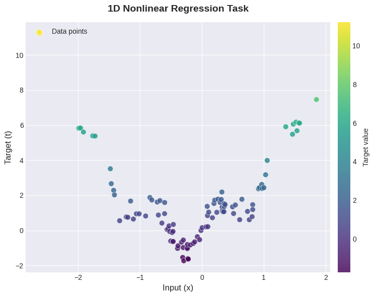
Training our Network

Now we get to see how our network performs on two concrete examples - a nonlinear synthetic dataset and the MNIST character recognition dataset. The synthetic regression dataset is visualised below.

Visualisation of the toy regression set — Figure 3. Visualisation of the toy nonlinear regression set.

We first have to decide some hyperparameters for each task:

Batch size $N$
Activation function
Number of layers
Neurons per layer
Number of epochs

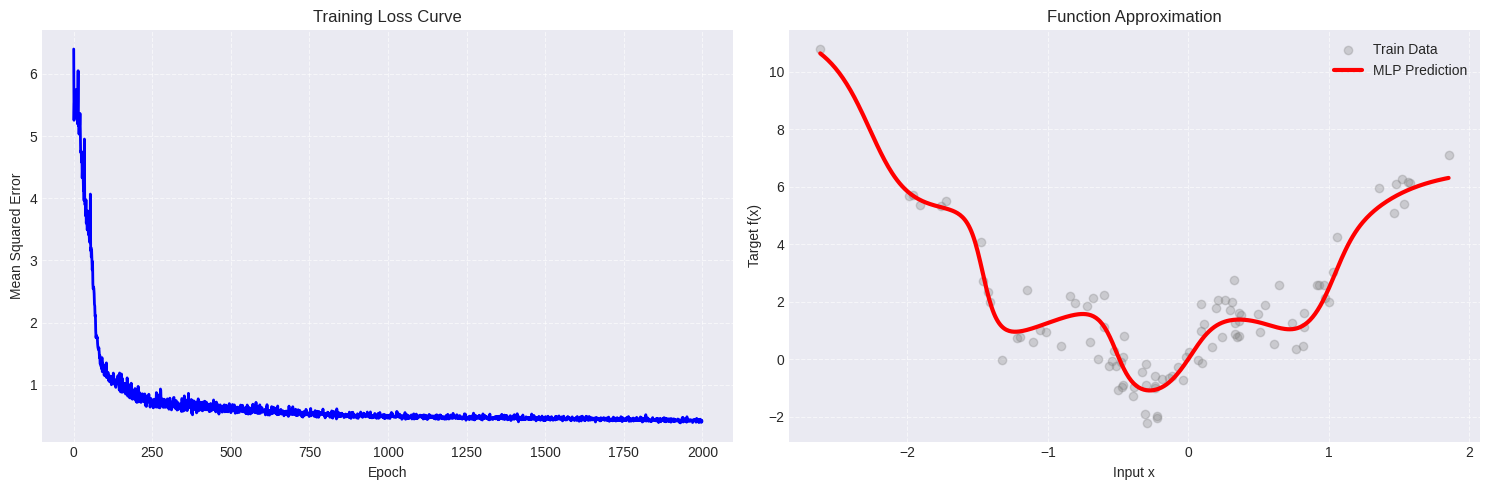
For the regression example, the following configuration seems to work welll:

batch_size = 8 
N_neurons = [16,8,4]
N_epochs = 2000

pbar = tqdm(range(N_epochs), desc="Training Progress")

mlp = MLP(N_features, N_neurons, K, task="regression", activations="sigmoid")
loss_history = []
for epoch in pbar:
    # random sample batches of data
    rand_idx = np.random.permutation(np.arange(N_samples))
    epoch_losses = []
    shuffled_data = data[rand_idx]

    for i in range(0,N_samples, batch_size):
        x_batch = shuffled_data[i:i+batch_size,0][:,None]
        t_batch = shuffled_data[i:i+batch_size,1][:,None]
        pred = mlp.forward(x_batch)
        loss = mlp.compute_loss(pred, t_batch)
        mlp.backward(pred, t_batch, eta=0.1)
        epoch_losses.append(loss)
    
    epoch_mean_loss = np.mean(epoch_losses)
    loss_history.append(epoch_mean_loss)
    pbar.set_postfix({"loss": f"{epoch_mean_loss:.6f}"})

Results visualisation — Figure 4. Visualisation network training on the regression task and predictions.

For the classification problem, we need sklearn to import the MNIST data. The image is comprised of 70k images, each with 28x28 dimensionality. Before we pass it to our network, we need to:

Split the data to train and test sets
Flatten the inputs
Apply a one-hot-encoding scheme to the labels for training.

The training loop is identical to the previous case.

mnist = fetch_openml('mnist_784', version=1, as_frame=False, parser='auto')
X_mnist, y_mnist = mnist.data, mnist.target.astype(int)

# Normalize pixel values to [0, 1]
X_mnist = X_mnist / 255.0

# One-hot encode labels for BCE loss
def one_hot_encode(labels, num_classes=10):
    one_hot = np.zeros((len(labels), num_classes))
    one_hot[np.arange(len(labels)), labels] = 1
    return one_hot

y_mnist_onehot = one_hot_encode(y_mnist)

# Train/test split (MNIST has 70k samples: 60k train, 10k test)
X_train, X_test = X_mnist[:60000], X_mnist[60000:]
y_train, y_test = y_mnist_onehot[:60000], y_mnist_onehot[60000:]
y_test_labels = y_mnist[60000:]  # Keep original labels for accuracy computation

mnist_batch_size = 64
mnist_neurons = [256, 128, 64]  # Larger network for image classification
mnist_epochs = 30
mnist_lr = 0.5

# Input/output dimensions
mnist_input_dim = 784  # 28x28 pixels
mnist_output_dim = 10  # 10 digit classes

# Instantiate MLP for MNIST
np.random.seed(42)
mnist_mlp = MLP(mnist_input_dim, mnist_neurons, mnist_output_dim, task="CE", activations="sigmoid")

# Training loop
mnist_loss_history = []
mnist_train_acc_history = []
n_train = X_train.shape[0]

pbar = tqdm(range(mnist_epochs), desc="MNIST Training")

for epoch in pbar:
    # Shuffle training data
    rand_idx = np.random.permutation(n_train)
    X_shuffled = X_train[rand_idx]
    y_shuffled = y_train[rand_idx]
    
    epoch_losses = []
    
    for i in range(0, n_train, mnist_batch_size):
        # Get batch
        X_batch = X_shuffled[i:i+mnist_batch_size]
        y_batch = y_shuffled[i:i+mnist_batch_size]
        
        # Forward pass
        pred = mnist_mlp.forward(X_batch)
        
        # Compute loss
        loss = mnist_mlp.compute_loss(pred, y_batch)
        epoch_losses.append(loss)
        
        # Backward pass and update
        mnist_mlp.backward(pred, y_batch, eta=mnist_lr)
    
    # Compute epoch statistics
    epoch_loss = np.mean(epoch_losses)
    mnist_loss_history.append(epoch_loss)
    
    # Compute training accuracy (every epoch)
    train_pred = mnist_mlp.forward(X_train[:5000])  # Subset for speed
    train_pred_labels = np.argmax(train_pred, axis=1)
    train_true_labels = np.argmax(y_train[:5000], axis=1)
    train_acc = np.mean(train_pred_labels == train_true_labels)
    mnist_train_acc_history.append(train_acc)
    
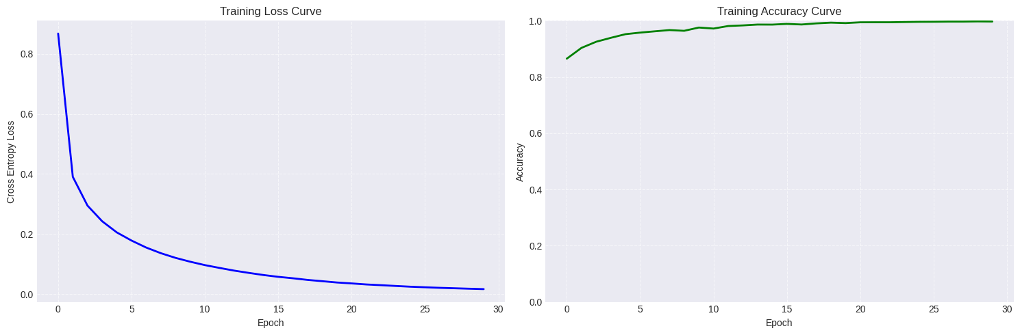
    pbar.set_postfix({"loss": f"{epoch_loss:.4f}", "train_acc": f"{train_acc:.2%}"})

Our model achieves an accuracy of 94.32% on the test set with a smooth loss curve as desired.

Classification results visualisation — Figure 5. Visualisation network training on the classification task with corresponding accuracy.

And there you have it! We have successfully implemented an MLP in pure numpy that generalises to regression, binary and multiple classification tasks. It all boils down to a sequence of affine transformations and some calculus that together form the backbone of modern deep learning.

The key takeaways from this post are:

Forward pass: Compute predictions via repeated affine transformations with nonlinear activations
Loss functions: Derived from maximum likelihood estimation, they measure how wrong our predictions are
Backpropagation: The chain rule applied systematically to compute gradients layer by layer
Optimisation: Iteratively nudge parameters in the direction that reduces the loss

While our implementation achieves respectable results on MNIST, production frameworks like PyTorch and JAX offer automatic differentiation, GPU acceleration, and optimised kernels that make training orders of magnitude faster. However, understanding these fundamentals will serve you well when debugging models, reading papers, or designing novel architectures.

In the next post, we'll extend these ideas to sequential data with Recurrent Neural Networks (RNNs), where the notion of "memory" becomes essential for tasks like language modelling and time series prediction.

Notes

Working on more complex tasks require some important considerations that are discussed below.

1. Weight initialisation

In the post above, we have initialised our network weights from a normal distribution. Weight initialisation has a big impact on how your network learns. See this Karpathy post on the relationship between activation functions and weight initialisation. Most DL frameworks use some varation of Kaiming uniform initialisation with ReLU and Xavier uniform for sigmoid/tanh activation. In the regression example above in particular, the wrong initalisation scheme when using ReLU activations led to pretty poor performance attributed to the dying ReLU problem.

2. Normalisation

Normalisation is crucial for stable and fast training in modern networks. There are two distinct aspects to consider:

Input/Output Normalisation: Before training, it's common to standardise inputs to zero mean and unit variance, or scale them to a fixed range like $[0, 1]$. This prevents features with large magnitudes from dominating gradient updates. Similarly, normalising regression targets can avoid large initial errors that cause exploding gradients.

Layer Normalisation Techniques: Several methods exist for normalising activations within the network:

Batch Normalisation (BatchNorm): Normalises across the batch dimension. Highly effective for CNNs, enabling higher learning rates and acting as a regulariser. However, it's sensitive to batch size and behaves differently at train vs. inference time.
Layer Normalisation (LayerNorm): Normalises across the feature dimension for each sample independently. The standard choice for Transformers and RNNs since it doesn't depend on batch statistics.

The choice depends on your architecture: BatchNorm for CNNs with reasonable batch sizes, LayerNorm/RMSNorm for Transformers and sequence models.

3. Numerical Stability

Production-grade neural network implementations include several numerical stability tricks that we glossed over in this post. Common techniques include: (1) clipping predictions before computing logarithms (e.g., np.clip(pred, 1e-7, 1-1e-7)) to avoid log(0) = -inf in cross-entropy losses; (2) the log-sum-exp trick for computing softmax, where you subtract the maximum value before exponentiating to prevent overflow (i.e., softmax(x) = exp(x - max(x)) / sum(exp(x - max(x)))); (3) gradient clipping to bound gradient magnitudes and prevent exploding gradients during backprop; and (4) adding small epsilon values to denominators in operations like layer normalisation or RMSprop to avoid division by zero. Modern frameworks like PyTorch and JAX handle many of these automatically, but understanding them is essential when debugging NaN losses or unstable training runs.